Experiments

This section documents the experiments conducted using the ETIA library.

Experimental Setup

We created synthetic data of 100, 200, 500, and 1000 nodes and an average node degree of 3. For the data generation, we assumed linear relationships and additive normal Gaussian noise. We used the Tetrad project for constructing random DAGs and data generation. We created 10 datasets of 2000 samples for each network size. In each DAG, we randomly selected a target variable (T) and one exposure variable (E) connected to the target with at least one directed path. For the following experiments, the true predictive model for these datasets is a linear regression model denoted as ( f ). For each repetition and network size, we also simulated hold-out data of 500 samples for the estimation of predictive performance in the AFS module.

AFS: Evaluating the Markov Blanket Identification

In the AFS module, we searched over twelve predictive configurations, consisting of two predictive learning algorithms (RF, linear regression), two feature selection algorithms (FBED, SES), and three significance levels (0.01, 0.05, 0.1). As in the case study, we searched for the Markov blanket (Mb) of T, ( M_b^{best}(T) ), the Mb of E, ( M_b^{best}(E) ), and the Mb of each node in ( M_b^{best}(T) ). We denoted the union of these sets as ( M_b^{best} ). The corresponding set ( M_b^{true} ) is determined by ( G_{true} ).

In Figure 1a, we plot the precision and recall of the ( M_b ) identification and the difference between the predictive performances (as measured by ( R^2 )), called ( Delta R^2 ), between the fitted model ( f(M_b^{best}(T)) ) returned by AFS and the optimal model ( f(M_b^{true}(T)) ) of the gold standard. The larger the difference, the worse the predictive model by AFS. Precision and recall are high for smaller network sizes, but precision decreases as the number of nodes increases. We obtained really few false-positive nodes while AFS did not miss many nodes that could be important in the next steps of the analysis (recall is above 0.80 even for 1000 nodes). The difference ( Delta R^2 ) shows that we obtained optimal predictive performance for the target regardless of the network size.

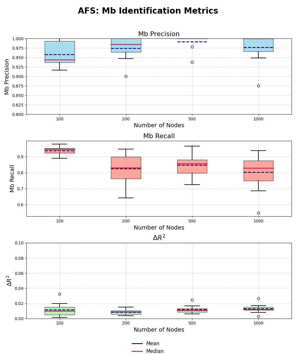
Figure 1a: Evaluation of the AFS module

CL: Evaluating the Output Causal Structure

The CL module returned the selected causal graph ( G_{M_b}^{est} ), where the superscript indicates that it is learned only from the variables returned by AFS. We compared this graph with ( G_{M_b}^{true} ), which is the marginal of the true graph over the variables of the true ( M_b ). The OCT tuning method in the CL module searched over six causal configurations, consisting of two causal discovery algorithms (FCI, GFCI) and three significance levels (0.01, 0.05, 0.1), and returned the selected graph ( G_{M_b}^{est} ).

In the first two rows of Figure 1b, we show the precision and recall of the adjacencies (i.e., edges ignoring orientation) in the output ( G_{M_b}^{est} ). As we increased the network size, adjacency precision remained relatively stable above 0.8 while the recall had a decrease for more tha 100 nodes. This aligns with previous results on ( M_b ) identification. In the last row (Figure 1b), we evaluated the tuning performance of OCT, and we plotted the difference in SHD (Structural Hamming Distance) between the optimal and the selected causal configuration. SHD counts the number of steps needed to reach the true PAG from the estimated PAG. As a result, SHD reflects both adjacency and orientation errors. OCT could select an optimal configuration in many cases. We noted that ( Delta SHD ) was low for small networks but slightly increased for larger networks due to larger SHD differences among the causal configurations.

Conclusion

These results demonstrate the robustness of our automated causal discovery process using ETIA across various synthetic datasets. Even with increasing network sizes, our methods maintained high precision in identifying Markov blankets, though recall tended to decrease. Future work will involve enhancing our methods to better handle large networks and improve the accuracy of causal effect estimations.